Introduction
Exploiting graph theory to grasp biological complexity
In Biology, form shapes function. The functioning of biological systems is tightly connected to their organization: trophic relationships among species,
cell-to-cell signals exchange, protein-to-protein interactions are only a few examples of the dynamic character of nature,
which perfectly orchestrates these events among all those that make the complex and fascinating network of life.
Network Biology exploits the foundamentals of mathematics and Graph Theory to tackle the complexity of natural systems. Networks (or Graphs)
are widely used to represent the dynamical interactions of such systems, where pairs of nodes are linked by edges, to represent
the existence of any relationship between them. Nodes and edges can be enriched with information in the form of attributes such as weights or edge directionality.
As a consequence and according to the nature and availability of these information, networks can be directed or weighted graphs.
For more information on this topic, please refer to this review by
Barabási and Oltvai.
Understanding the team-play effect of groups of nodes using mesoscale indices
Centrality is the proxy for the definition of core properties of networks. It is estimated by means of several mathematical indices, which can be divided into two main categories:
- Global indices: to measure properties that concern the whole graph and that recall its organization and topological structure. For example, the average shortest path length measures the average distance between every pair of nodes in a graph; it can be considered as a measure of the speed of information flow and used as a metric of efficiency.
- Local indices: to explore the specific properties of a single node or edge. For example, the degree of a node is measured as the number of edges incident to the node. Despite being the simplest metrics, it is widely used to quantify the extent of nodal connectivity of a graph and is a cornerstone of network analysis.
Although powerful, global and local indices fail to capture any joint effect of nodes
and their systemic interplay. In cell biology in fact, the majority of cellular functions
are fulfilled by groups of genes, each playing a peculiar and defined role in the observed
biological process. Programmed cell death, for example, is a multifaceted, intracellular process
that requires the cooperative effects of many genes to start, as there is no single upstream
gene that can start the apoptotic cascade. These genes often do not interact directly with
each other, rather they act on overlapping gene sets and transcription factors to
exert their function.
It is common knowledge, however, that the components of a biological network are functionally
related, even if not directly interacting. This implies that their underlying interaction
network might exhibit nodes not directly connected to each other, but that are functionally
related instead. Hence, finding critical members of functionally active groups of nodes is a crucial aim that
requires proper mathematical indices. To do that, we first extended the concepts of degree, closeness and
betweenness centrality to groups of nodes and, then, we defined ways to identify key player nodes
within a graph (Borgatti, 2006).
Why should I use Pyntacle?
Pyntacle makes the double-job of making common methods for biological network analysis available off-the-shelf, as well as of providing efficient implementations of algorithms for the discovery of team-play effects. This is done by means of reformulations of centrality indices which apply to groups rather than to individual nodes, and of advanced algorithms for the identification of key player sets of nodes.
↑ backGroup centrality as an extension of local centrality metrics
This class of topological indices is a strict extension of that of their homonym local centrality indices,
since they are applied to groups rather than to individual nodes. Differently from local metrics,
a group centrality score applies to an array of nodes taken together, neglecting the contributions of the
individuals. It is straightforward to notice that these indices can be useful also in Biology, other than
in Social Sciences, where these were born from.
The group centrality metrics implemented in Pyntacle are group degree, group closeness
and group betweenness. They were firstly described by Everett and Borgatti in a paper that dates back to 1999
(https://doi.org/10.1080/0022250X.1999.9990219).
Pyntacle stays faithful to the definitions reported in this paper, but the reader must be warned that
other formulations of these metrics exist in literature.
Group degree
Group degree is defined as the number of non-group nodes |N \ X| of a graph G that are connected to the node set X. In this formulation, multiple ties between X and the other nodes are counted once. This number is then normalized by the the total number of non-group nodes, deriving the following formula:
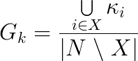
where kappa is the number of non-redundant ties between X and the rest of the graph.
Group degree ranges from 0 to 1, where 0 means that the group is completely disconnected
from the rest of the graph and 1 means that the node set reaches all nodes in the graph.
If we consider the toy network in Fig. 1, for example, the node set {a,b} reaches all the
remaining nodes in the network (6/6), hence its group degree is 1.

Fig. 1
Group closeness
Group closeness is the the sum of the distances from the group X to all the other nodes N\X. Since this formulation produces an inverse measure of closeness as larger numbers indicate less centrality, the final closeness is normalized by dividing it into the total number of non-group nodes:
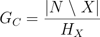
where d(x,C) is the shortest possible distance between the group and the non-group node x. The
definition of distance is customizable. It can be set as the minimum, maximum and
average distance between group and non-group nodes.
Group betweenness
Group betweenness counts the proportion of shortest paths connecting pairs of non-group members that pass through the group, divided by the total number of geodesics connecting those pairs.
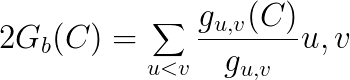
This formula is normalized by dividing it by the theoretical maximum, i.e. (|N \ X|)(|N \ X|-1):
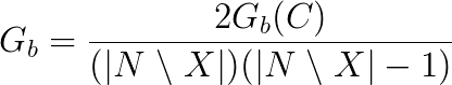
where N is the size of the graph and X is the size of the group.
↑ backIdentifying key players in biological networks
Other topological metrics exist that can be applied to groups, which do not rely on common local centrality
indices. We focus here on those that tackle the Key Player Problems, as formulated by S. Borgatti in
https://doi.org/10.1007/s10588-006-7084-x.
-
The first problem is called the Negative Key Player Problem (KPP-NEG) and regards the issue of
identifying the group of nodes that maximally fragment a network;
-
The second problem, or the Positive Key Player Problem (KPP-POS), concerns the problem of searching the
nodes that are reachable by the majority of other nodes.
Fragmentation (KPP-Neg): how to efficiently disrupt a network
The Negative Key Player problem (KPP-Neg) aims at finding the smallest possible set of nodes whose removal would maximally disrupt a network. Two metrics exist that face this problem: F and dF. The former accounts for the number of components created upon removal of a set of nodes, while the latter captures the relative cohesion of the residual components.
F
F measures the fragmentation of a network by looking at the number of network components and their
sizes. It is defined as:
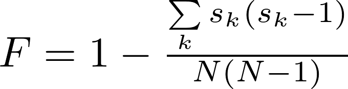
where N is the number of nodes, and sk is the size (number of nodes)
of the kth component.
F ranges
from 0 to 1. If a network has only one component, F = 0. If a network consists of only isolates, F = 1.
dF
dF is a global metrics that measures the distance-based fragmentation of a network. It is defined as:
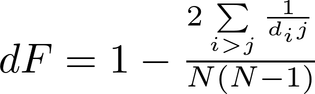
where N is the number of nodes, and dij is the distance (shortest path) between any nodes i and j in the network. As for F, dF ranges from 0 to 1.
↑ backImportant remarks
Why and when to resort to fragmentation metrics
Degree and betweenness centrality can be used to assess the overall network cohesion. However, there are cases where these may dramatically fail. Consider for example the toy network in Fig. 2 (taken from the original article by Borgatti). Node degree and node betweenness agree to consider node 1 as the best option to fragment the network. However, this choice does not cause a dramatic disconnection of the network. A link between nodes 7 and 8 survive and keeps the total number of components to 1. In contrast, removing node 8 does create two components, although not exhibiting highest centrality values.
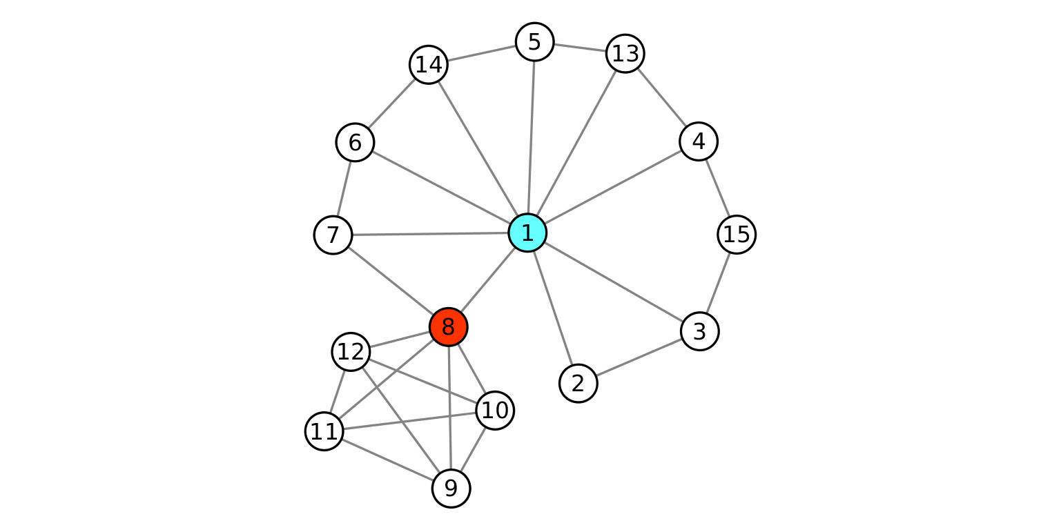
Fig. 2
Known Limitations
The "No Fragmentation" issue
- If the removal of a set of nodes does not increase the number of components of a network, the F value will not change.
- Biological networks are in general more resilient to fragmentation than other real networks. This might be due to their high redundancy that, in turn, works protecting from different types of perturbation (e.g., mutational, environmental). Robust traits, as modularity, bow-tie architectures, degeneracy, and other topological features, cooperate to reduce the number of effective perturbations. Robustness is a topological property and is linked to the network density only marginally. Removing the only edge connecting two groups of dense nodes might in fact be critical and thus cause the fragmentation of the network.
- The robustness property has an important implication in the search of the best kp-set: robust networks might be less affected by the removal of even the best node set, since this might cause a minimal or no fragmentation, thereby leaving the fragmentation score almost unchanged.
The “Network Size” issue
The formulation of dF includes the calculation of the shortest paths between any pair of nodes in a network. If the strategy to find the best kp-set encased the calculation of dF for all (or many) candidate kp-sets, this might be computationally demanding and time-consuming. Calculating dF on large networks (>103 nodes) may take hours or days, depending on structural features of the networks like, e.g., the network's density. Multicore/GPU computing were exploited to alleviate the overall computational load and increase algorithmic performance.
↑ backReachability (KPP-Pos): How to efficiently spread information across a network
Imagine to be a social media analyst working for a small company. The company is about to launch a
new software and asks you to find the ideal targets (bloggers, youtubers, etc) to which granting early
access to the software. Beta-testers must be few and very popular. Who would you choose?
This is the Positive Key Player problem (KPP-Pos) and can be reformulated as follows:
Given a graph G, with N nodes and l links, what is the subset k of n that can reach
as many remaining nodes as possible via direct links or short paths?
To this aim, we implemented the m-reach and dR metrics.
m-reach
m-reach is a reachability measure that counts how many unique nodes can be reached from a kp-set in m steps or less, where m is the maximum distance (shortest path) between the kp-set and the remaining nodes. Its formulation is:
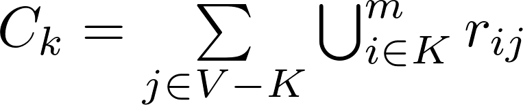
where m is the maximum allowed shortest path distance between the node i belonging to the kp-set and any node j outside of it, and r is a reachability matrix, where rij = 1 if i can reach j via a path of length m or less, and rij = 0 otherwise. M-reach ranges from 0 to N-K, with N being the total number of nodes and K the size of the set. The disadvantage of this measure is that it assumes that all paths of length m or less are equally important and that all paths longer than m are wholly irrelevant.
↑ backdR
dR stands for distance-weighted reach and bases its formulation on the measure of the distances (shortest paths) between the node set and the remaining nodes in the graph. It is defined as:
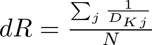
where N is the total number of nodes in the graph and dKj is the minimum distance between any member i of the kp-set and the remaining nodes in the graph. For convenience of interpretation, all distances within the kp-set members are considered to be zero. For example, let us consider the node 1 and 7 being part of the kp-set of the graph in Fig. 3
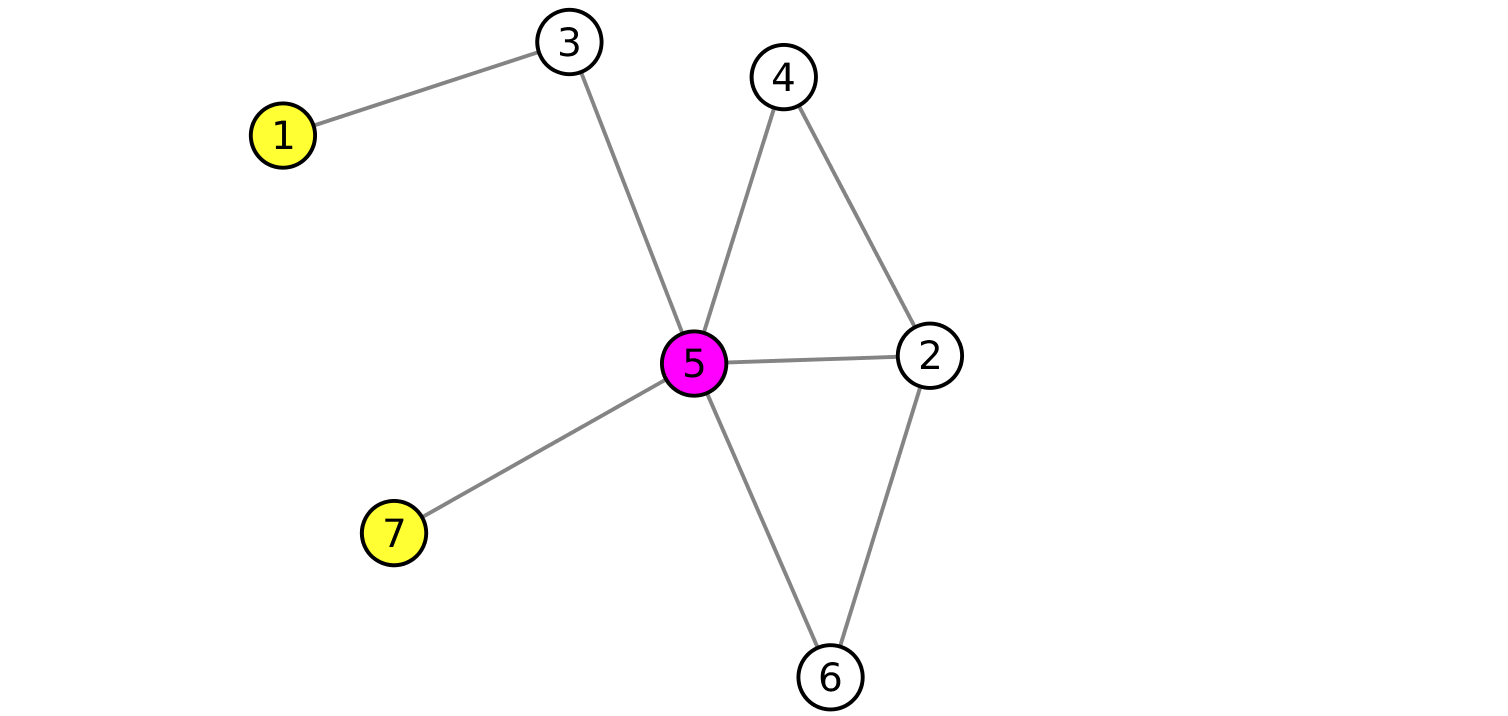
Fig. 3
The distances between the kp-set and the node 5 is 1, since 1 is the length of the shortest path from any
member of the kp-set.
Similarly, dK,3 = 1, dK,4 = 2,
dK,2 = 2, dK,6 = 2.
Hence, dR ranges from 0 and 1. It is 0 when the kp-set is completely disconnected from the other nodes.
It is 1 when the kp-set can reach all other nodes of the network.
Important remarks
Why and when to resort to reachability metrics
Closeness centrality is a reachability metrics. However, even if node 4 of the graph in Fig. 4 has the highest closeness measure, it is not the most central node in terms of reachability, since it reaches 6 nodes with 2 links or less, while node 3 can reach 8 nodes with 2 links or less.
Fig. 4
The conclusion is that canonical metrics may provide optimal, but not the best solutions, that can be explored with reachability-inspired metrics, like the m-reach or dR. Contrary to fragmentation, which is a global measure, reachability is local to a set of ndoes.
↑ backSearch strategies of for group centrality assessment
All the group metrics described here can be computed by both command line and using the Pyntacle APIs.
Measuring the centrality of a set of nodes
Group centrality, fragmentation and reachability of a selected set of nodes can be computed by using
the gr-info and the kp-info arguments of pyntacle groupcentrality
and pyntacle keyplayer command line tools of Pyntacle and by specifying the node names by the
--nodes parameter. Octopus APIs include the following methods to perform the same job: kp_F,
kp_dF, kp_mreach and kp_dR.
Optimization search strategies
When the aim is finding the best node set in terms of group centrality indices, fragmentation or reachability, Pyntacle provides two optimization search strategies: the greedy optimization and the brute-force search algorithms.
Greedy optimization
Greedy optimization is a heuristics that aims at finding an optimal group of nodes, which may not
necessarily be the best set for a predefined centrality metrics. It works by first selecting a group
of nodes of size k, and then by swapping every member in the node set with each other nodes in the
graph until there is no set with a better centrality value. Greedy optimization is the default method
in the gr-finder and kp-finder command line tool for the
pyntacle groupcentrality and pyntacle keyplayer commands, respectively. Using the APIs,
this search method can be invoked by first importing GreedyOptimization class which is located in
the algorithms.greedy_optimization module or through the GO group of methods of
Octopus.
Brute-force search
Brute-force search aims at finding all the best groups that maximize a given group metric. It
simply enumerates all possible sets of nodes of a predefined size and calculates the selected centrality measure
for them. Finally, it ranks all sets and returns the best solutions. Despite its simplicity, this algorithm is
computationally demanding and time consuming. For this, it was implemented to exploit multi-core
processors.
Brute-force search can be enabled using the bruteforce option of the --implementation
parameter of gr-finder and kp-finder command line tools.
Programmatically, it can be run by the
BruteforceSearch class in the algorithms.bruteforce_search module
or by calling the BF group of methods of Octopus.