 Pyntacle Quickstart Guide
Pyntacle version 1.0
Table of Contents
- Introduction
- Setting Pyntacle for the first use
- Dataset Description
- Command line Startup Guide
- Pyntacle library startup guide
- Import a network using Pyntacle
Octopus: A convenient wrapper of Pyntacle methodsOctopus: Compute key player metrics for a given set of nodeOctopus: Greedy optimization searchOctopus: Brute-force search- Export the
igraph.Graphobject for external use - Key player search without
Octopus: Brute-force search (case example)
Introduction 
In this brief tutorial, we will show you how to use Pyntacle to find relevant groups of nodes (also called here the kp-set) in a network using the key player metrics of fragmentation and reachability.
Fragmentation is the effect of removing nodes on the communication and structure of a network. Reachability is the property of nodes to reach their direct or indirect neighbors in a network. Although we will provide here a brief explanation of these concepts, we recommend to first read the introduction to group centrality section for brief overview.
This guide will help using Pyntacle both from your command shell and as a Python library. All data used in this tutorial are available here for download.
Setting Pyntacle for the first use 
After installing Pyntacle as described in installation instructions, you must enter into the pyntacle environment by typing
conda activate pyntacle_env
Note: pyntacle_env is just a naming convention, you can name the environment however you want.
You can then find the binary files by typing in your shell:
which pyntacle
For example, this is the location of the Pyntacle’s binaries on a Linux Mint 18 system where Pyntacle was installed through Conda:
/home/d.capocefalo/miniconda3/bin/pyntacle
Alternatively, you may run Pyntacle through our Docker Image or build a custom Pyntacle Docker Image using our Dockerfile.
If using Pyntacle as a Python library, typing:
import pyntacle
on a python3 shell will end with no error if Pyntacle was successfully installed. Otherwise, contact us and send us a description of the error, along with all the necessary information to reproduce your error.
Dataset Description 
The toy dataset is the network of advice-seeking ties among global consulting companies (also called in this tutorial the AdvSeek network). This network was already used in the original paper by Stephen P. Borgatti, in which key player metrics are introduced, Identifying sets of key players in a social network .
The network can be represented as follow
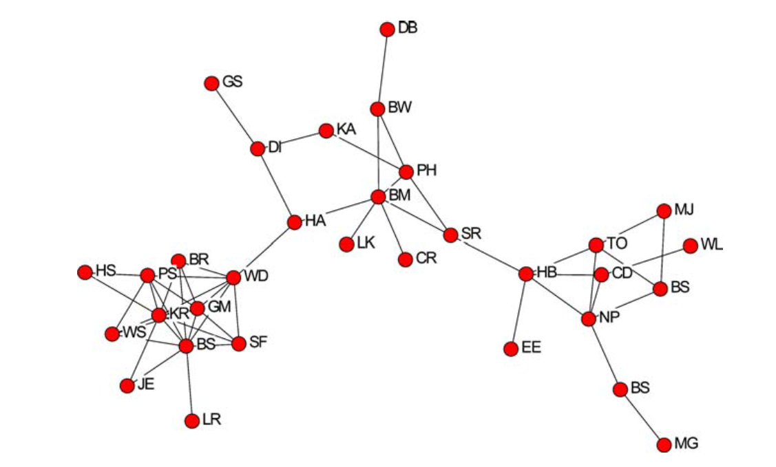
We made this network available here as an adjacency matrix (one of our supported file formats). Nodes in the network are labeled with the initials of the consultants. Since some of the consultants share the same initials, we appended progressive numbers to their initials (e.g. BS, BS2, BS3, etc) to be compliant with the Pyntacle Minimum Requirements. Edges represents relationships among consultants.
Command line Startup Guide 
Testing the Pyntacle Command Line 
To check that Pyntacle is properly installed and working, a set of unit tests can be run by typing in the command shell:
pyntacle test
Pyntacle will perform several operations that will end with a similar message no errors will be encountered.
Ran 23 tests in 1.002s
OK
<pyntacle.pyntacle.App object at 0x7f7c22f8be10>
Otherwise, please contact us specifying your operative system, its version, how you installed Pyntacle and the output of your tests in a text file. You can redirect the output of the Pyntacle tests this way:
pyntacle test >> testlog.txt 2>&1
Once verified the correct installation of Pyntacle, we replicated some of the results of Borgatti’s original article in two steps.
kp-info: Compute key-player metrics for a given set of nodes 
As a first step, the Pyntacle kp-info module will be used to measure the dF measure (a fragmentation index) for a specific node set of the AdvSeek network. Borgatti measured the dF value of the pair {HB, WD} and obtained a value of 0.817. We recall here that dF ranges from 0 to 1, when 0 means maximum connectedness (i.e., the network is a clique) and 1 means maximum disconnection (all nodes are isolates). This result can be replicated by typing:
pyntacle keyplayer kp-info -i AdvSeek.adjm -t dF --nodes HB,WD
This command returns the following output on your shell (we report the final summary only for the sake of readability):
Nodes given as input: ['HB', 'WD']
Computing dF for nodes HB,WD
Elapsed Time: 0.00 sec
Keyplayer metric(s) DF:
Starting value for dF is 0.64755. Removing nodes ['HB', 'WD'] gives a dF value of 0.81506
Producing report in txt format.
Generating plots in pdf format.
Pyntacle Keyplayer completed successfully. Ending
The resulting fragmentation can be better assessed comparing the dF of the original network (before removal) with that calculated after the removal of the set. For this reason, the kp-info module returns also the dF value of the original network.
Results of the kp-info module can be saved in several file formats (default is the tab-separated value file format), along with a graphical network representation, when the network is small enough to be clearly represented in a picture (generally in the order of hundreds of nodes). These plots will be stored in a sub-directory, pyntacle-plots, of the current working directory.
Note: you can redirect both the report and the plots to a custom directory, using the --directory/-d argument.
The representation of the AdvSeek network follows where the removed nodes were represented in purple.
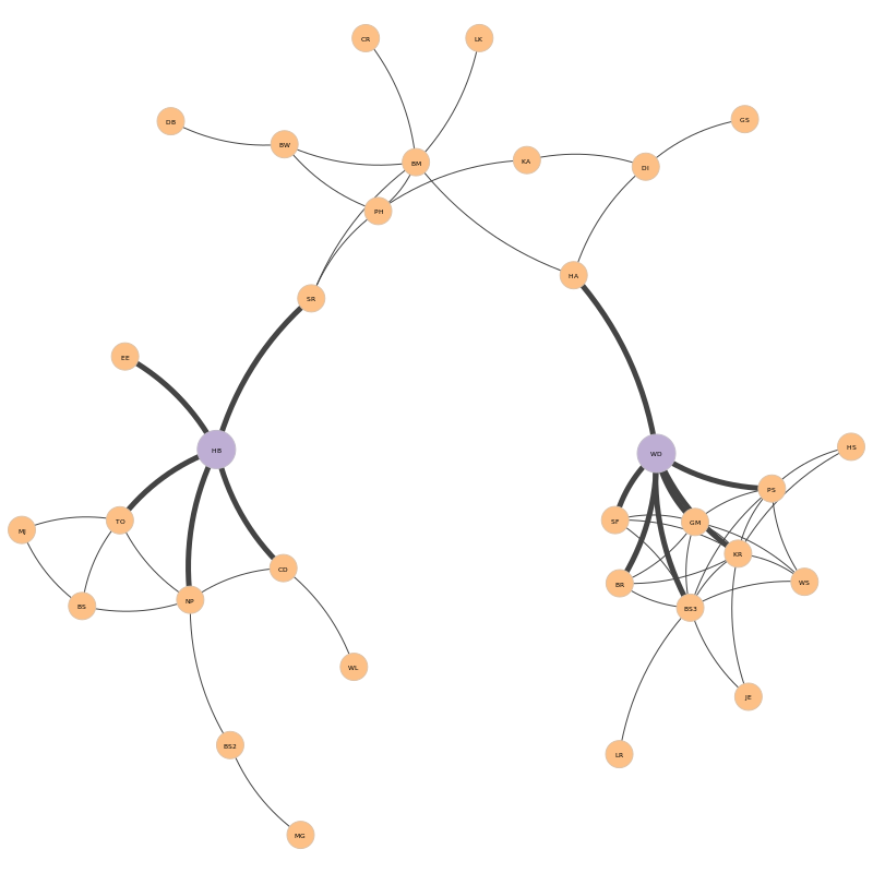
(Thicker edges around the kp-set highlight the {HB, WD} neighborhood)
kp-finder: Greedy optimization search 
In case one wants to find the set of nodes of a particular size that maximally fragments the network or reaches the highest number of other nodes, a greedy optimization algorithm was implemented. It may not obtain the best unordered set of nodes of size k for the selected metrics, since this task would require:
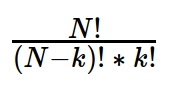
operations, where N is the size of the graph. Starting from a random set of nodes and then swapping nodes with others outside the set until the key player metrics cannot be improved, one dramatically reduces the number of operations at the cost of suboptimal solutions. This algorithm is particularly useful when dealing with large networks, in the order of thousands or tenth of thousands of nodes, like a whole interactome.
The key player metric chosen in this tutorial is the m-reach, which is a measure of reachability. It aims at counting the number of nodes reached by a vertex set of size k in m steps or less. In Borgatti’s paper, the m-reach metric is calculated on the AdvSeek network two different ks, with a maximal m of 1
| k | Nodes reached | % of network reached | kp-set |
|---|---|---|---|
| 2 | 17 | 53 | {BM, BS3} |
| 3 | 23 | 72 | {BM, BS3, NP} |
Note: The node BS is here called BS3 as there are 3 synonymous nodes in the original graph)
To reproduce this result, type:
pyntacle keyplayer kp-finder -i AdvSeek.adjm -k 2 -m 1 -t mreach --seed 100
The kp-finder enables the use of the greedy optimization search algorithm by default. This behavior can be changed using the -I/--implementation argument and setting the brute-force option (See the brute-force section). The --seed argument ensures results reproducibility, as the random initial set selection and node swapping will always be the same.
Pyntacle will output:
****************************************** RUN SUMMARY *******************************************
Node set size for key player search: 2
Key player set of size 2 for positive key player index m-reach, using at best 1 steps is:
(BS3, BM)
with value 15 on 32 (number of nodes reached on total number of nodes)
The total percentage of nodes, which includes the kp-set, is 53.12%
****************************************************************************************************
Note: We report the number of only the nodes reached by the kp-set (m-reach) and the percentage of reached nodes, which includes the kp-set (as from Borgatti’s paper).
Results are stored in a txt file in the current working directory, together with a visual plot that will highlight the nodes being part of the resulting kp-set. Thickness of edges will decrease as the distance from the kp-set (m) will increase.
Similarly, the optimal set of size 3 can be sought typing:
pyntacle keyplayer kp-finder -i AdvSeek.adjm -k 3 -m 1 -t mreach --seed 1
This will produce the following output (again, only the run summary is reported):
****************************************** RUN SUMMARY *******************************************
Node set size for key player search: 3
Key player set of size 3 for positive key player index m-reach, using at best 1 steps is:
(KR, BM, NP)
with value 20 on 32 (number of nodes reached on total number of nodes)
The total percentage of nodes, which includes the kp-set, is 71.88%
****************************************************************************************************
The resulting kp-set {KR, BM, NP} is not the same reported by Borgatti {BM, BS3, NP}, despite their scores being identical. This means that this network holds more kp-sets of size 3 with equal fragmentation scores.
A way of getting all these sets would be to run the greedy optimization search algorithm several times. But this will not guarantee to capture all existing kp-sets. Another, exact, way would be to switch to the Brute-force search algorithm, as we will discuss in the next section.
kp-finder: Brute-force search 
Contrary to the greedy optimization search algorithm, the brute-force search algorithm seeks and finds the best solutions at the price of high demand of computing resources and running times. However, it was implemented to calculate the desired metrics for all combinations of size k of nodes in parallel on multiple CPUs, if available. The brute-force algorithm can be enabled by setting the -I/--implementation parameter with the brute-force keyword. By default, Pyntacle will use all available computing cores minus one (e.g. 7 cores out of 8 in an octacore processor). However, this can be tuned by the -T/--threads parameter.
Let's consider again the AdvSeek network and the case discussed in the previous chapter. The greedy optimization search did not replicate Borgatti's findings on the AdvSeek network. Searching again the best kp-sets of size 3 with the brute-force search algorithm:
pyntacle keyplayer kp-finder -i AdvSeek.adjm -k 3 -m 1 -t mreach -I brute-force
Note: The brute-force algorithm does not need to specify a seed, because it will always converge to the best solutions.
****************************************** RUN SUMMARY *******************************************
Node set size for key player search: 3
Key player sets of size 3 for positive key player index m-reach, using at best 1 steps are:
(KR, BM, NP)
(BS3, BM, NP)
with value 20 on 32 (number of nodes reached on total number of nodes)
The total percentage of nodes, which includes the kp-set, is 71.88%
****************************************************************************************************
The two best solutions were finally found. This concludes the quick start guide of Pyntacle via command line. The same problems will be tackled using Pyntacle as a Python library in two fashions: by means of the Octopus wrapper and by directly using the Pyntacle Methods for kp-search.
Pyntacle library startup Guide 
The library is designed for intermediate-to-expert python users with a basic knowledge of object oriented programming and some experience with the igraph package (not necessarily for python, as igraph bindings are available also for the C and R languages). If you are not acquainted with igraph basics, we recommend reading its official Python tutorial.
Pyntacle is built around igraph and perform its calculations on instances of igraph.Graph objects. Pyntacle provides several utilities for importing/exporting from/to igraph.Graph objects to/from several textual network file formats. We refer to the File Formats Specifications page for more details on regard. Moreover, we recommend reading the Minimum Network Requirements page to see whether your network can be parsed and used by Pyntacle.
Finally, a complete description of each class and method is available from our API Documentation page.
Import a network using Pyntacle 
Networks can be imported from file via the PyntacleImporter class of the io_stream module. This class contains a series of handy methods that parse and store an input graph into an igraph.Graph object and initialize all the Pyntacle reserved attributes (see the Minimum Network Requirements section).
Considering again the AdvSeek network, which is available as an adjacency matrix from file “AdvSeek.adjm”, it is imported with the following command:
from pyntacle.io_stream.importer import PyntacleImporter

adv = PyntacleImporter.AdjacencyMatrix("AdvSeek.adjm")
It is an igraph object
type(adv)
and can exploits all the built-in igraph functions.
The adv object can be also inspected by means of standard igraph methods:
adv.summary()
Octopus: A convenient wrapper of Pyntacle methods 
The classes and methods used to perform all the operations described in the Command Line Guide are not encompassed into a single module, but they are rather divided in appropriate sub-methods, that can be recalled (see the API documentation, algorithms section). A handy wrapper of all these methods is the Octopus class. It is contained in the tools module. The list of all the Octopus methods can be inspected:
from pyntacle.tools.octopus import Octopus

dir(Octopus)
When calling an Octopus function on an igraph object, Octopus will execute the corresponding Pyntacle function and will assign a new attribute to the graph with the result of the function as a value. For example, let's suppose one wants to compute the average degree of the AdvSeek network. Typing:
Octopus.add_average_degree(adv)
will trigger the computation of the average degree, will create an average_degree attribute for the graph and will set the result (3.4375 for the AdvSeek Network) to it:
adv.attributes()
adv["average_degree"]
Octopus: Compute key player metrics for a given set of nodes 
Let's say we want to reproduce Borgatti's results for network fragmentation on the AdvSeek network we already discussed in the corresponding Command Line Section. We can do this using Octopus like in the following example
Octopus.add_kp_dF(adv, nodes=["HB", "WD"])
Where nodes is a list of names of the nodes belonging to the kp-set.
Octopus will add a new attribute, dF_kpinfo, to the graph adv. This attribute is actually a dictionary, where each item is a key, value pair made by a (sorted) tuple of nodes (the kp-set) and the corresponding dF value. This naming convention stands for each of the key player metrics we implemented.
adv.attributes()
and
adv["dF_kpinfo"]
dF is a relative metrics, in the sense that the effect of removing a set can be appreciated if compared with the fragmentation level of the original network. The initial dF value of a network we can be computed by using the add_DF method
Octopus.add_dF(adv)
The initial dF is stored in the corresponding dF attribute
adv["dF"]
Now, we can conclude that removing HB and WD will result in an increase in fragmentation of 17%.
Octopus: Greedy optimization search 
The previous greedy optimization, which was performed by the command line kp-finder command, can be replicated with the add_GO_mreach method.
Octopus.add_GO_mreach(adv,kp_size=2, m=1, seed=100)
Like in the previous section, Octopus adds an attribute to the graph that stores a dictionary of node names (kp-set) and centrality measures. In this example, the attribute will be called mreach_1_greedy, since the centrality metrics is the m-reach with m=1 argument and obtained with a run of the greedy optimization search algorithm
adv.attributes()
The name is as much informative as possible. It shows that the m-reach metric with an m distance of 1 was searched with the greedy optimization criteria. This ensures that all the greedy optimization searches for m-reach of distance 1 will be stored here, keeping tracks of all the runs.
As before, we can see the corresponding dictionary keys and their values associated to them
adv["mreach_1_greedy"]
Octopus: Brute-force search 
Finally, the brute-force search performed through the command line can be replicated with Octopus using the maximum number of available computing cores minus one.
Octopus.add_BF_mreach(adv, kp_size=3, m=1)
Again, we can see that a new attribute storing the brute-force search is stored into the adv object. This attribute is stored in the mreach_1_bruteforce attribute. This attribute will contain a tuple of 3 storing the node names as key and the corresponding m-reach value. This attribute does not overlap with the other key player searches we performed, to ensure a different layer of information for each search.
adv["mreach_1_bruteforce"]
Export the igraph.Graph object for external use 
Any igraph.Graph can then be saved to a textual file (we refer again to the File Formats Specifications page) or a binary file. Additionally, graphs can be exported with all their attributes. The export utilities are implemented in the PyntacleExporter class of the io_stream module.
Let's export the adv network into a binary format:
from pyntacle.io_stream.exporter import PyntacleExporter

PyntacleExporter.Binary(adv, "AdvSeek.graph")
This will return a file named advseek.graph in our current directory (we print the full path by default).
Key player search without Octopus: Brute-force search (case example) 
The same operations performed with Octopus can also be performed by resorting to the Pyntacle APIs (algorithms and tools modules). These methods rely on an array of enumerators by which specifying:
- the key-player metrics to be calculated;
- the computing modes for some of the Pyntacle’s methods (i.e., serial, parallel CPU, parallel GPU);
These enumerators are implemented in the tools module and can be imported as:
from tools.enums import KpposEnum #this enumerator stores all the reachability metrics
from tools.enums import CmodeEnum #this one handles all the implementations
KpposEnum currently includes two reachability metrics: m-reach and dR.
dir(KpposEnum)
CmodeEnum contains four values: auto, igraph, cpu and gpu; auto is the default choice and commands Pyntacle to choose the best computing mode, according to the specific features of the graph is working on. The igraph value is chosen if one relies on the single-core implementations of igraph of some algorithms underlying the Pyntacle’s methods, while cpu is used when one relies only on Pyntacle functions, the computationally heavy ones being just-in-time compiled by Numba and run in parallel on multicore processors. Finally, gpu is used to defer computationally heavy functions to be executed on CUDA-enabled NVIDIA graphics cards, if available. The value of this enumerator can be passed to the implementation parameter of any key-player methods.
dir(CmodeEnum)
For example, the brute-force search executed before with Octopus can be replicated using the BruteForceSearch method this way:
from pyntacle.algorithms.bruteforce_search import BruteforceSearch as bfs
bfs.reachability(graph=adv, implementation=CmodeEnum.igraph, kp_type=KpposEnum.mreach,m=1,kp_size=3)
This concludes our Quick Startup guide. If you want to leave a feedback, please contact us